
1. Backpropagation
1.1 Theory and Examples
The perceptron learning rule of Frank Rosenblatt and the LMS algorithm of Bernard Widrow arid Martian Hotf were designed to train single-layer perceptron-like networks. these single-layer networks suffer from the disadvantage that they are only able to solve linearly separable classification pmhlems. Both Rosenblatt and Widraw were aware of these limitations and purposed multilayer networks that could overcome them, but they were not able to generalize their also-rithms to train these more powerful networks.
Apparently the first description of an algorithm to train multilayer networks was contained in the thesis of Paul Werhos in 1974. This thesis presented the algorithm in the context of general networks, with neural networks as a special case, and was not disseminated in the neural
network community. It was not until the mid 1980s that the backpropaga-tion algorithm was rediseovered and widely publicized. It was rediscovered independently David H.umelhart, Geoffrey Hintan and Ronald WilHams,David Parker and Yann Ixe Cun. The algo-rithm was popularized its inclusion in the book Parndled Distributed Pro-teas, which described the work afthe Parallel Dixtributed Processing Group led psychologists David Rumelhart and James Mc-Clelland. The publication of this book spurred a torrent of research in neu-ral networks. The multilayer perceptmn, trained by the backprapagation algorithm, is currently the most widely used neural network.this chapter we will first investigate the capabilities of multilayer net works and then present the barkpropagation algorithm.
1.2.1 Muitilayer Perceptrons
We first introduced the notation for multilayer networks. Forease of reference we have reproduced the diagram of the three-Iayer perceptron in Figure 1-1. Note that we have simply cascaded three perceptrop networks. The output of the first network is the input to the second network, and the output of the sevond network is the input to the third net-work. Each layer may have a different number of neurons, and even a different transfer function. we are using superecripts to identify the layer number. Thus, the weight matrix for the first layers written as W1 and the weight matrix for the second Layer is written W2.
To identify the structure of a multilayer network, we will sometimes use
the following shorthand notation, where the number of inputs is followed
by the number of neurone in each layer:
R – S1 - S2 - S3

Figure 1.1 Three-Laver Network
Let's now investigate the capabilities of these muitilayer peroeptron net-works. first we willlook at the use of multilayer networks for pattern classificativn, and then we wi11 discuss their application to Function
approximation.
1. Pattern Classificatian
To illustrate the capabilities of the multilayer perception for pattern classification,consider the classic exclusive-or(XOR) problem.The inputltarget pairs for the XOR gate are

This problem, which is illustrated graphically in the figure 1-2, was used by Minsky and Papert in 1969 to demonstrate the limitations of thesingle-layer perceptmn. Because the two categories are not linearly separuble, a single-layer perceptron cannot perform the classification.

Figure 1-2
A two-iayer network can solve the XOR problem. In fact, there are many different multilayer solutions. One snlntian is to use two neurons in the first lever to create two decision boundaries. The first boundary separates P1, from the outer patterns, and the second boundary separates P4. Then the second layer is used to combine the two boundaries together using an AND operation. The decision boundaries for each first-layer neuron are shown in Figure 1-3.

Figure 1.3 Decision Boundaries for XOR Network
The resulting two-layer, 2-2-1 network is shown in Figure 1-4. The overalldecision regions far this network are shown in the figure in the left margin.The shaded region indicates those inputs that will produce a network output of 1.

Figure 1.4 Two-Layer XOR Network
See Problems P1.1 and P1.2 for mare an the use of multilayer networks
for pattern classification.
2. Function Approximation
Up to this point in the text we have viewed neural networks mainly in the context of pattern classification. It is also instructive to view networks as function approximators. In control systems, far example, the objective is to find an appropriate feedback function that maps from measured outputs to control inputs.In adaptive filtering the objective is to find an that maps from delayed values of an input signal to an appropriate output signal. the following example will illustrate the flexibility of the multilayer perceptron for implementing functions.
Consider the two-Iayer,1-2-1 network shown in Figure 1.5. For this example the transfer function for the first layer is log-sigmoid and the transfer function for the second Layer is linear. In other words,
 and
and 
Suppose that the nominal values of the weights and biases for this network are
 ,
, ,
, ,
, ,
, ,
, ,
,

Figure 1.5 Example Funetion Apprnximatioa Network
Tie network respaose for these parameters is shown in Figure 1.5, which plots the network output as a2 input P is varied over the range [-2, 2].
Notice that the response consists of two steps, one for each of the lag-sigmold neurons in the First layer.By adjusting the network parameters we can change the shape and location of each step, as we will see in the following diseussion.
The centers of the steps occur where the net input to a neuron in the first
layer is zero:


The steepness of eacn step can he adjusted by changing the network weights.

Figure 1.6 Nominal Response of Network of Figure 1.5
Figure 1.7 illustrates the effects of parameter changes on the network respouse. The blue curve is the nominal response. The other curves correspond to the network response when one parameter at a time is varied over the fallowing ranges:
 ,
, ,
,
Figure 1.7 shows how the network biases in the fist (hidden) Iayer can be used to locate the position of the steps. Figure 1.7 (b) illustrates how the weights determine the slope of the steps. The bias in the second (out put) layer shifts the entire network response up or down, as can be seen in figure 1.7(d).From this example we can see how flexible the multilayer network is. It would appear that we could use such networks to approximate almost any function, if we had a sufficient number of neurone in the hidden layer. In fact, it hss been shown that two layer networks, with sigmoid transfer functions in the hidden layer and linear transfer functions in the output
layer, ran approximate virtue any function of interest to any degree of accuracy, provided sufficiently many hidden units are available .

Figure 1.7 Effect of Parameter Changes an Network Response
1.2.2 The Backpropagation Algorithm
It will simplify our development of the backpropagation algorithm if we use the abbreviated notation For the multilayer network, The three-layer network in abbreviated notation is shown inFigure 1.8.
As we discussed earlier, for multilayer networks the output of one layer becames the input to the following layer. The equations that describe this。
 ,
, 1.6
1.6
where M is the number of layers in the network. The neurons in the first
Iayer receive external ixsputs:
 1.7
1.7
which pmr}ides the starting point for Eq(1.8). The outputs ofthe neurons in tha last layer are considered the network outputs:
 1.8
1.8

Figure 1-8 Three-Layer Network, Abbreviated Notation
1.2.3 Performance Index
The hsckpropagatian algorithm for multilayer networks is a generalization
of the LMS algorithm, and both algorithms use the same per fomance index: mean square error. The Algorithm is pravided with a set of exampe of proper network behavior.
 1.9
1.9
where Pq is an input to the network, and tq is the corresponding target output. As each input is applied to the network, the network output is compared to the target. The algorithm should adjust the network parameters in order to minimize the mean square error:
 1.10
1.10
where X is the vectar of network weights and biases.If the network has mutltiple outputs this generalizes to
 1.11
1.11
As with the LMS algorithm, we will approxmate the mean square error by
 1.12
1.12
where the expectation of the squared error has been replaced by the squared error at iteration k.
The steepest descent algorithm far the approximate mean square error is
 1.13
1.13
 1.14
1.14
where  is the learning rate.
Sa far, this development is identical to that for the LMS algorithm. Now we come to the difficult part-the computation of the partial derivatives.
3. Chain Rule
Far a single-layer linear network (the ADALINE) these partial derivatives
are conveniently computed using. Far the multilayer network the error is not an explicit function of the weights in the hidden layers, therefore these derivatives are not competed so easily.
Because the error is an indirect function of the weights in the hidden layers, we will use the chain rule of calculus to calculate the derivatives. To review the chain rule, suppose that we have a funtion f that is an explcit function only of the variable n We want to take the derivative of f with respect to a third. variable w . The chain rule is then:
 1.15
1.15
For example,if
 OR
OR  , so that
 1.16
1.16
Then
 1.17
1.17
We will use this oancept to find the derevatives and Eq.(1.13)and(1.14):
 1.18
1.18
 1.19
1.19
The second term in earn of these equations can be easily computed, since the net input to layer m is an explicit function of the weights and bias in that layer:
 1.20
1.20
Therefore
 1.21
1.21
If we now define
 1.22
1.22
(the serasitiuity of  to changes in the ith element of the net input at layer m ), then Eq.(1.18)and Eq.(1.9) can be simplified to
 1.23
1.23
 1.24
1.24
We can naw express the approximate steepest descent algorithm as
 1.27
1.27
 1.28
1.28
Where
 1.29
1.29
4. Backpropagating the Sensitivities
It now remains for us to compute the sensitivities Sm,which requires another application of the chain rule. It is this process that gives us the term, backpropigation, because it describes a recurrence relationship in which the sensitivity at layer m is computed from the sensitivity at layer m+1.
To derive the recurrence relationship for the sensitivities, we will use the following Jacobian matrix:
 1.30
1.30
Next we want to find an experssion for this matrix. Consider the i,j element of the matrix:

 1.31
1.31
Where
 1.32
1.32
Therefore the Jacobian matrix can be written
 1.33
1.33
Where
 1.34
1.34
We can now write out the recurrence relation far the sensitivity by using
the chain rule in matrix form:
 1.35
1.35
Now we can see where the backpropagatinn algorithm derives its name.
The sensitivities are propagated backward through the network from the
last layer to the first layer:
 1.36
1.36
At this point it is worth emphasizing that the backgropagation algorithm uses the same approximate steepest descent technique that we used in the LMS aigorithm. The only eomplication is that in order to compute the gradiem we need to first backpropagate the sensitivities. The beauty of backpropagation is that we have a vary efficient implemsntatinn of the chain rule.
We still have one more step to make in order to complete the backpropagation algorithm. We need the starting point,SM,for the recurrence relation of Eq.(1.35).This obtained at the final layer:
 1.37
1.37
Now,since
 1.38
1.38
we can write
 1.39
1.39
This can be expressed in matrix form as
 1.40
1.40
5. Summary
Let's summarize the backprogagation algorithm. The first steg is to propagate the input forward through the network:
1.41
 1.42
1.42
1.43
The nest step is to propagate the sensitivities backward through the net
work:
1.44
 1.45
1.45
Finally, the weights and biases are updated using the approximate steepest descent rule:
 1.46
1.46
1.47
1.2.3 Example
To illustrate the backprapagatiom algorithm, let's choose a network and apply it to a particular problem. To begin, we will use the 1-2-1 network that we discussed earlier in this chapter. For convenienoe we have reproduced the network in Figure 1-8.
Next we want to define a problem for the network to sole. S want to use the network to approximate the function
 1.48
1.48
To obtain our training set we will evaluate this Function at several values
of p.

Figure 1-8 Exampe Function Approximation Network
Before we begin the backpropagation algorithm we need to some initial values for the network weights and biases. Generally these are chosen to be small random values. In the next chapter we will discuss some rea sons for this. For now let's choose the values

The response of the network far these initial values is illustrated in Figure 1-9, along with the sine function we wish to appmromate.

Figure 1-9 Initial Network Response
Now we are ready to start the algorithm. For our initial input we will choose p=1:

The output of the first layer is then


The second layer output is

The error would then be

The next stage of the algorithm is to barkprapagate the sensitivities.Before we begin tha backpmpagation, recall that we will need the derivatives of the transfer functions,  and
and  . For the first layer

FOr the second Iayer we have

We can now the backprapagation. The starting point is found at the second layer, using Eq.(1.4).

The first layer sensitivity is then computed by backpropagating the sensitivity from the second layer, using Eg.(1.45).

The final stage of the algorithm is to update the weights. For simplicity, we will use a learning rate a=0.1.From Eq.(1.46)and Eq.(1.47)we have


This completes the first iteration of the backpropagativn algorithm. We next proceed to choose another input p and perform another iteration of the algorithm. We continue to iterate until the difference between the network response and the target function reachces some acceptable level. We will discuss convergence criteria in more detail in Chapter 2.
1.2.4 Using Backpropagation
In this section we will present some issues relating to the practical implemantation of backpropagation. We will discuss the choice of network architecture, and problems with network convergence and generalization.
1. Choice of Network Architecture
As we discussed earlier in this chapter, multilayer networks can be used to approximate almost any function, if we have enough neurons in the hidden layers. However, we cannot say, in general, haw many layers or how many neurone are necessary for adequate performance, In this section we want to use a few examples to provide some insight into this problem.
For our first example let's assume that we want to approximate the following functions:
 1.49
1.49
where i takes on the values 1, 2, 4 and 8. As i is increased, the function
becomes more complex, because we will have more periods of the sine wave
over the interval  .It will be more difficult far a neural network
with a fixed number of neusrons in the hidden layers to approximate g ( p)
as I is increased.
Far this first example we will use a 1-3-1 network, where the transfer funetion for the first layer is log-sigmoid and the transfer function for the second layer is linear. this type of two-layer network can produce a response that is a sum of three log-sigmaid functions (or as many log-sigmoids as there are neurons in the hidden layer). clearly there is a limit to how complex a function this network can implement. Figure 1-10 illustrates the response of the network after it has been trained to approximate g (p) for i = 1, 2, 4, 8 .The final network reaponaea are shown by the blue lines.

Figure 1-10 Function Approximation Using a 1-3-1 Network
We can see that for i=4 the 1-3-1 netwark reaches its maximum capahil ity. When i>4 the network is not capable of prnducing an accurate apprnx imation of g(p).In the bottom right graph of Figure 1-10 we can see how the 1-3-1 network attempts to approximate g(p)for i=8 .The mean square error between the network response and g(p)is minimized, but the network response is only able to match a small part of the function.
In the next example we will approach the problem from a slightly different
perspective. This time we will pick one function g (p) and then use larger
and larger networks until we are able to accuratelyc9epresent the function. For g (p) we will use
 1.50
1.50
To approximate this function we will use two-layer networks, where the
transfer function for the first layey is log-sigmoid and the transfer function for the second layer is linear (1-S1-1 networks). As we discussed earlier in this chapter, the response of this network is a superposition of S1 sigmoid functions.
Figure 1-11.illustrates the network response as the number of neurons in the first layer (hidden layer) is increased. Unless there are at least eve neurons in the hidden layer the network cannot accurately represent g(p).

Figure 1-11 Effect of Increasing the Number of Hidden Neurons
To summarize these results, a 1-S1-1. network, with sigmoid neurons in the hidden layer and linear neurons in the output layer, can produce a re sponse that is a superposition of S1 sigmoid functions. If we want to op proximate a function that has a 1arge number of inflection points, we will need to have a large number of neurons in the hidden layer.
2. Convrergence
In the precious section we presented same examples in which the network
response did not give an accurate approximation to the desired function,
even though the backpropagation algorithm produced network parameters
that minimized mean square error. This occurred because the capahilities
of the network were inherently limited by the number of hidden neurons it contained. In this section we will provide an example in which the network is capable of approxiamating the function, but the learning algorithm does not produce network parameters that produce an accurate approximation. In the next chapter we will discuss this problem in more detail and explain why it occurs. For now we simply want to illustrate the problem.
The function that we want the network to approximate is
 1.51
1.51
To approximate this ,unction we will use a 1-3-1 network, where the transfer function for the first layer is log-sigmoid and the transfer function for the second layer is Linear.
Figure 1-12 illustrates a case where the learning algorithm converges to a solution that minimizes mean square error. The thin blue lines represent intermediate iterations, and the thick blue line represents the final solution, when the algorithm has converged. (The numbers next to each curveindicate the sequence of iterations, where 0 represents the initial condition and 5 represents the final solution. The numbers do not correspond to the iteration number. There were many iterations for which no curve is nepreaerated. The numbers simply indicate an ordering.)

Figure 1-12 Convergence to a Global Minimum
Figure 1-13 illustrates a case where the learning algorithm converges to a solution that does not minimize mean square error. The thick blue line (marked with a 5) represents the network response at the final iteration.
The gradient of the mean square error is zero at the final iteration, there fore we have a local minima, but we know that a better solution exists, as evidenced by Figure 1-12. The only difference between this result and the resultt shown in Figure 1-12 is the initial condition. From one initial condition the algorithm converged to a global minimum point, while from another initial condition the algorithm converged to a Iocal nunimum paint.

Figure 1-13 Convergence to a Lacal Minimum
Note that this result could not have occurred with the LMS algorithm. The Mean square error performance index for the ADALINE network is a qua dratic function with a single minimum point (under most conditions).
Therefore the LMS alsrorithm is guaranteed to conversge to the global minimum as long as the learning rate is small enough. The mean square Error for the multilayer network is generally much more complex and has many local minima (as we will see in the next chapter). When the backprapagation algorithm converges we cannot be sure that we have an optimum so lotion. It is best to try several different initial conditions in order to ensure that an optimum solution has been obtained.
3. Generalization
In most cases the multilayer network is trained with a finite number of examples of proper network behairior:
1.52
This training set is normally representative of a much larder clash of possibale input output pairs. It is important that the network successfully generahaze what it has learned to the total population.
For example, suppose that the training set is obtained by sampling the following function:
1.53
at the points p=-2,-1.6,-1.2,…,,1.6 ,2。(There are a total of 11 input/target pairs.) In Figure1-14 we see the response of a 1-2-1 network that has trained on this data. The black line represents g(p),the blue line represents the network response, and the ‘+’symbols indicate the training set.

Figure1-14 Network Approximation of g (p)
We can see that the network response is an accurate representation of (p).If we were to find the response of the network at a value of p that as not contained in the training set(e.g.,p=-0.2),the network would till produce an output close to g(p).This network generalizes well.Now consider Figure 1-15, which shows the response of a 1-9-1 network hat has been trained on the same data set. Note that the network response ccurately models g(p) at all of the training points. However, if we compute the network response at a value of p not contained in the training set (e.g.p=-0.2)the network might produce an output far from the true response g(p).This network does not generalize well.

Figure 1-15 1-9-1 Network Approximation of g(p)
The 1-9-1 network has too much flexibility for this problem; it has a total f 28 adjustable parameters (18 weights and 10 biases), and yet there are nly 11 data points in the training set. The 1-2-1 network has only 7 parameters and is therefore much more restricted in the types of functions hat it can implement.
Far a network to be able to generalize, it should have fewer parameters than there are data points in the training set. In neural networks, as in all modeling problem,we want to use the simplest network that can adequately represent the training set. Don't use a bigger network when a smaller network (a concept often referred to as Ockham’s Razor).
An alternative to using the simplest network is to stop the training before
the network overfits. A reference to this procedure and other techniques to improve generalization.
2 variations on Backpropagation
2.1 Objectives
The backpropagation algorithm introduced in Chapter 1 was a major breakthrough in neural network research. However, the basic algorithm is too slow for moat practical applications. In this chapter we present several variations of backpropagation that provide significant speedup and make the algorithm more practical.
We will begin by using a function approximation example to illustrate why the baekpropagation algorithm is slow in converging. Then we will present several modifications to the algorithm. Recall that backpropagation is an approximate steepest descent algorithm.we saw that steepest descent is the simplest, and often the slowest, minimization method. The conjugate gradient algorithm and Newton’s method generally provide faster convergence. In this chapter we will explain how these faster procedures can be used to speed up the convergence of backpropagation.
2.2 Theory and Examples
When the basic backpropagation algorithm is applied to a practical problem the training may take days or weeks of computer time. This has encouraged considerable research on methods to accelerate the convergence of the algorithm.
The research on faster algorithms falls roughly into two categories. The first category involves the development of heuristic techniques, which arise out of a study of the distinctive performance of the standard baekpropagation algorithm. These heuristic techniques include such ideas as varying the learning rate, using momentum and resealing variables. In this chapter we will discuss the use of momentum and variable learning rates.
Another category of research has focused on standard numerical optimization techniques. As we have discussed in Chapters 1, training feedforward neural networks to minimize squared error is simply a numerical optimization problem. Because numerical optimization has been an important research subject for 30 or 40 years, it seems reasonable to lack for fast training algorithms in the large number of existing numerical optimization techniques. There is no need to "reinvent the wheel" unless abaoIute1y necessary. In this chapter we will present two existing numerical optimization techniques that have been very successfully applied to the training of multilayer perceptrons: the conjugate gradient algorithm and the Levenherg-Marquardt algorithm (a variation of Newton's method).
We should emphasize that all of the algorithms that we will describe in this chapter use the backpropagation procedure, in which derivatives are processed from the last layer of the network to the first. For this reason they could all be called "backpropagation" algorithms. The differences between the algorithms occur in the way in which the resulting derivatives. Used to update the weights. In same ways it is unfortunate that the algorithm we usually refer to as backpropagation is in fact a steepest descent algorithm. In order to clarify our discussion, for the remainder of this chapter we will refer to the basic backpropagation algorithm as steepest descent backpropagation (SDBP).
In the next section we will use a simple example to explain why SDBP has problems with convergence. Then, in the following sections, we will present various procedures to improve the convergence of the algorithm.
Drawbacks of Backpropagation
Recall from Chapter 1 that the LMS algorithm is guaranteed to converge to a solution that minimizes the mean squared error, so long as the learning rate is not too large. This is true because the mean squared error for a single-layer linear network is a quadratic function. The quadratic function has only a single stationary point. In addition, the Hessian matrix of a quadratic function is constant, therefore the curvature of the function in a given direction does not change, and the function contours are elliptical.
SDBP is a generalization of the LMS algorithm. Like LMS, it is also an approximate steepest descent algorithm for minimizing the mean squared error. In fact, SDBP is equivalent to the LMS algorithm when used on a single-layer linear network. When applied to multilayer networks, however, the characteristics of SDBP are quite different .This has to du with the differences between the mean squared error performance surfaces of single-layer linear networks and multilayer nonlinear networks. While the performance surface for a single-layer linear network has a single minimum paint and constant curvature, the performance surface far a multilayer network may have many local minimum points, and the curvature can vary widely in different regions of the parameter space .This will becorne clear in the example that follows.
Performance 5urtace Example
To investigate the mean squared error performance surface for multilayer networks we will employ a simple function approximation example. We will use the 1-2-1 network shown in figure 12.1, with log-sigmoid transfer functions in both layers.

Figure 2-1 Function Approximation Netwvrk
In order to simplify our analysis, we will give the network a problem far which. we know the optimal solution, The function we wilt approximate is the response of the same 1-2-1 network, with the following values for the weights and biases:
, ,
, , 2.1
, 2.1
 ,,,
,,, 2.2
2.2
The network response for these parameters is shown in Figure 12.2, which plots the network output a2 as the input p is varied over the range[-2,2].

Figure 2-2 Nominal Function
We want to train the network of Figure 2-2o approximate the function displayed in Figure 2.2. The approximation will he exact when the network parameters are set to the values given in Eq. (2.1)and Eq. (2.2).This is, of course, a very contrived problem, but it is simple and it illustrates same important contents.
Let's now consider the performance index for our problem. We will assume that the function is sampled at the values
 2.3
2.3
and that each occurs with equal probability. The performance index will be the sum of the squared errors at these 41 points. (We won't bother to find the mean squared error, which just requires dividing by 41.)
In order to he able to graph the performance index, we will vary only two parameters at a time. figure 12.3 illustrates the squared error when only  ,
, are being adjusted, while the other parameters are set to their optimal values given in Eq. (2.1) and Eq. (2.2). Note that the minimum error will be sera, and it wilt occur when and,as indicated by the open blue circle in the figure.
There are several features to notice about this error surface. First, it is clearly not a quadratic function. The curvature varies drastically over the parameter space. For this reason it will be difficult to choose an appropriate learning rate far the steepest descent algorithm. In some regions the surface is very flat, which would allow a large learning rate, while in other regions the curvature is high, which would require a small Learning rate. (Refer to discussions in and 10 on the choice of learning rate for the steepest descent algorithm.)
It should be noted that the flat regions of the performance surface should not be unexpected, given the sigmoid transfer functions used by the network. The sigmoid is very flat far large inputs.
A second feature of this error surface is the existence of more than one local minimum point. The global minimum point is located at and along the valley that runs parallel to the axis. However, there is also a local minimum, which is located in the valley that runs parallel to the asis. (This local minimum is actually off the graph at 
 ) In the next section we will investigate the perfarmance of backprapagation on this surface.

Figure 2-3 Squared Error Surface Versus and
Figure 2.4 illustrates the squared error when and  are being adjusted, while the other parameters are set to their optimal values. Note that the minimum error will be zero, and 1t will occur when and =-5 as indicated衍the open blue circle in the figure.
Again we find that the surface has a v ery contorted shape, steep in some regions and very flat in others. Surely he standard steepest descent algo rithm will surface. For example, if we have an initial guess of  ,=-10 the gradient will be very dose to zero, and the steepeat descent algorithm would effectively stop, even though it is not close to a local minimum paint.

Figure 2-4 Squared Error Surface Versus and
Figure 2.5 illustrates the squared error when 和 are being adjusted, while the other parameters are set, to their optimal values. The minimum error is located at =-5 and
  as indicated by the open blue circle in the figure.
This surface illustrates an important property of multilayer networks: they have a symmetry to thenn. Here we see that there are two local minimum paints and they bath have the same value of squared error. The second soIution corresponds to the same network being turned upside dawn (i.e., the top neuron in the first layer is exchanged with the bottom neuron). It is because of this characteristic of neural networks that we as not set the initial weights and biases to xero. The symmetry causes zero to be a saddle point of the performance surface.
This brief study of the perfarmance surfaces for multilayer networks gives us same hints as to haw to set the initial guess for the Sl)BP algorithm.First, we do not want to set the initial parameters to zero. This is because the origin of the parameter space tends to be a saddle point for the performanta surface. Second, we do not want to set the initial parameters to large values. This is because the performance surface tends to have very flat regions as we move far away from the optimum point.
Typically we choose the initial weights and biases to be small random values. In this way we stay away from a gvssible saddle point at the origin without moving out to the very flat regions of the performance surface. As we will see in the next section, it is also useful to try several different initial guesses, in order to be sure that the algorithm converges to a global minimum paint.

Figure 12.5 Squaxed Error Surface Versus and
2.2 Convergence Example
Now that we have examined the performance surface, let's investigate the performance of SDBP. For this section we will use a variation of the standard algorithm, called batch ing, in whieh the parameters are updated only after the entire training set has been presented. The gradients calculated at each training example are averaged together to produce a mare accurate estimate of the gradient. ( If the training set is complete, i.e., covers all possible inputJautput pairs, then the gradient estimate will be exact. )
In Figure 2-6 we see two trajectories of SDBP (batch made) when only two parameters, and are adjusteu. For the initial condition labeled “a” the algontnm does eventually converge to the convergence is the change in curvature of the surface over the path of the trajectory. After an initial into a very gently sloping valley. If we were to increase the learning rate, the algorithm would converge faster while passing over the initial flat surface, but would become unstable when failing into the valley, as we will see in a moment.
Trajectory “b”illustrates how the algorithm can converge to a local minimum point. Ttie trajectory is trapped in a valley and diverges from the optimal solution.If allowed to continue the trajectory converges to ,.The existence of multiple lncal minimum points is typical of the performance surface of multilayer networks. For this reason it is best to several different initial gueases in order to ensure that a global minimum has been obtained. (Some of the local minimum points may have the same value of squared error, as we saw in Figure 2-5, so we would not expect the algorithm to converge to the same parameter values for each initial guess. We just want to be sure that the same minimum exror is obtained.)

Figure 2-6 Two SDBP (Batch Mode) Trajectories
The progress of the algorithm can also be seen in Figure 2.7, which shows the squared error versus the iteration number. The curve on the left corresponds to trajectory “a”and the curve on the right corresponds to trajectory “b”These curves are typical of SDBP, with Iong periods of little progress and then short periods of rapid advance.

Figure 2-7 Squared Error Convergence Patterns
We can see that the flat sections in Figure 2.7 correspond to times when the algorithm is traversing a flat section of the performance surface, as shown in Figure 2-6. During these periods we would like to increase the learning rate,in order to speed up convergence. However, if we increase the learning rate the algorithm will become unstable when it reaches steeper portions of the performance surfaee.
This effect is illustrated in Figure2-8. The trajectory shown here corresponds to trajectory "a" in Figure 2-6, except that agarger learning rate was used. The algorithm converges faster at first, but when the trajectory reaches the narrow nailey that contains the minimum point the algorithm being to diverge. This suggests that it would be useful to vary the learning rate. We could increase the learning rate an that surfaces and then decrease the learning rate as the slope increased. The question is: How will the algorithm know when it is an a flat surface? We will discuss this in a later section.

Figure 2-8 Trajectory with Learning Rate Too Large
Another way to improve convergence would be to smooth out the trajectory .Note in Figure 2.8 that when the algorithm begins to diverge it is oscillating back and forth across a narrow valley. If we could filter the trajectory,by averaging the updates to the parameters, this might smooth out the oscillations and produce a stable trajectory, We will discuss this procedure in the next section.
2.3 Heuristic Modifications of Backpropagation
Now that we have investigated some of the drawbacks of backpropagation (steepest dent), let's consider some procedures far improving the algorithm. In thus section we will discuss two heuristic methods. In a later seetion we will present two methods based on standard numerical optimixation algoritluns.
1. Momentum
The first method we will discuss is the use of momentum. This is a modification based on our observation in the last section that convergence might be impmved if we could smooth out the oscillations in the trajectary. We can do this with a low-pass filter.
Before we apply momentum to a neural network application, let's investigate a simple example tv illustrate the smoothing effect. Consider the following first-order filter:
 2.4
2.4
Where  is the input to the filter,
  is the output of the filter and
  is the momentum wefficient that must satisfy.
 2.5
2.5
The efl'ect of this filter is shown in Figure 2.9. For these examples the input to the Filter was taken to be the sine wave:
 2.6
2.6
and the momentum coefficient was set to =0.9 (left graphy ) and = 0.98
(right graph). Here we~see that the oscillation of the filter output is less than the oscillation in the filter input (as we would expect for a low-pass filter). In addition, as y is increased the oscillation in the filter output is reduced. Notice also that the average filter output is the same as the average filter input, although as y is increased the filter output is slower to respond.

Figure 2.9 Smoothing Effeet of Momentum
Ta summarise, the filter tends to reduce the amount of oscillation, while still tracking the average value. Now let's see how this works an the neural network problem. First, recall that the parameter updates for SDBP (Eq.(1.46) and Eq. (1.4'l)) are
 2.7
2.7
 2.8
2.8
When the momenturrz filter is added to the paxameter changes, we obtain the following equations far the m8mentum modification to backpropagation (MOBP):
 2.9
2.9
 2.10
2.10
If we now apply these modified equations to the example in the preceding section, we obtain the results shown in Figure 2.10. (For this example we have used a batehing form of MOBP, in which the parameters are updated only after the entire training set has bean presented. The gradients calculated at each training example are averaged together to produce a mare accurate estimate of the gradient.) This trajectory corresponds to the same initial condition and learning rate shown in Figure 2.8, but with a momentum coeffcient of =0.8,We can see that the algorithm is now stable. By the use of momentum we have been able to use a larger learning rate,while maintaining the stability of the algorithm. Another feature of momentum is that it tends to accelerate convergence when the trajectory is moving in a consistent direction.
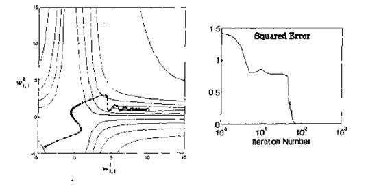 Figure 2-10 Trajectory with Momentum
If you Iook caref, ully at the trajectory in Figure 2.10, you can see why the procedure is given the name mornentum. It tends to make the trajectory continue in the same direction. The larger the value of r, the mare “momentum” the trajectory has.
2. Variable Learning Rate
We suggested earlier in this chapter that we might be able to speed up convergence if we increase the learning rate on flat surfaces and then decrease the learning rate when the slope increases. In this section we want to explore this cancept.
Recall that the ruean squared error performance surface for single-layer linear networks is always a quadratic function, and the Hessian matrix is therefore constant. The maximum stable learning rate for the steepest descent algorithm is two divided by the maximum eigenvalue of the Hessian matrix. (See Eq. (1.25).)
As we have seen, the error surface far the multilayer network is not a quadratic function. The shape of the surface can he very different in different regions of the parameter space. Perhaps we can speed up convergence by adjusting the learning rate during the course of training. The trick will be to determine when to change the learning rate and by how much.
There are many different approaches for varying the learning rate. We will describe a very straightforward hatching procedure [VaMa$8], where the learning rate is varied according to the performance of the algorithm. The rules of the variable Learning rite backprapagation algorithm (VLBP) are:
1. If the squared error (aver the entire training set) increases by more than some set percentage (typically one to five percent) after a weight update, then the weight update is discarded, the learning rate is multiplied by some factor 0<P<1,and the momentum coeffcient (if it is used) is set to zero.
2. If the squared error decreases after a weight update, then the weight update is accepted and the learning rate is multiplied by same factor If y has been previously set to zero; it is reset to its original value.
3. If the squared error increases by leas than ,then the weight update is accepted but the learning rate is unchanged. If has been previousIy set to zero, it is reset to its original value.
To illustrate VLBP, let's apply it to the function approximation emblem of the previous section. Figure 2.11 displays the trajectory fur the algorithm using the same initial guess, initial learning rate and momentum coefficient as was used in Figure 12.10. The new parameters were assigned the values.
 =1.05,
 =0.7,=4% 2.11

Figure 2-11 Variable Learning Rate Trajectory
Notice how the learning rate, and therefore the step sire, tends to increase when the trajectory is traveling in a straight line with constantly decreasing error. This effect can also be seen in Figure 2.12, which shows the squared error and the learning rate versus iteration number.
When the trajectory reaches a narrow galley, the learning rate is rapidly decreased. otherwise the trajectory would have become oscillatory, and the error would have increased dramatically. For each potential step where the error would have increased by more than 40, the learning rate is reduced and the momentum is eliminated, which allows the trajectory to make the quick turn to fallow the valley toward the minimum point. The learning rate then increases again, which accelerates the convergence. The learning rate is reduced again when the trajectory overshoots the minimum point when the algorithm has almost converged. This process is typical of a VLBP trajectory.

Figure 2.12 Convergence Characteristics of Variable Learning Rate
There are many variations on this variable learning rate algorithm. Jacobs proposed the delta-bar-delta learning rule, in which each network parameter (weight or bias) has its own learning rate. The algorithm increases the learning rate for a network parameter if the parameter change has been in the earns direction for several iterations. If the direction of the parameter change alternates, then the learning rate is reduced. The Supers A,B algorithm of Tallenaere is similar to the delta-bar-delta rule, but it has mare complex rules for adjusting the learning rates,
Another heuristic modification to SDGP is the Quickprop algorithm of Fahlman, It assumes that the error surface is parabolic and concave upward around the minimum point and that the effect of each weight can be considered independent.The heuristic modifications to SIGP can often provide much faster oonvergence for some problems. However, there are two main drawbacks to these methods. The first first is that the madificatians require that several parameters be set (e.g., ,and ),while the only parameter requred far SDBP is the learning rate. Some of the more complex heuristic modifications can have five or six parameters to be selected often the performance of the algorithm is sensitive to changes in these parameters. The choice of paramters is also problem dependent.The second drawback to these modifications to SDBP is that they can sometimes fail to converge on problems for which SDBP will eventually find a solution. Both of these draw hacks tend to occur more often when using the more complex algorithms.


